Note: This post is a follow-up to another post I wrote, which is a more general introduction to heuristic optimization algorithms. I recommend you read my earlier post before this one.

I wrote this post with helpful input from the awesome ladies at a Chicago Write/Speak/Code meetup! Kara Carrell wrote a great post on The Four A’s, and I’ll link to what others wrote as it comes online.

Let’s say you have a optimization problem you want to solve. You can calculate how good a given solution is (you have a fitness function), but you don’t know anything about the fitness landscape. No problem; you can use a heuristic optimization algorithm to find a solution. Maybe you’ve already chosen an algorithm to work with (say, simulated annealing). Now you’re good to go, right? Time to run it and get the solution you need?

Well, not exactly. Turns out, if you actually want to use heuristic optimizers, you have a lot of decisions to make, and lot of things to tune. Here are the ones you’ll run into over and over:

1. Stop conditions (number of steps/run time)
2. Fixed parameters or parameter sets (mutation rate for genetic algorithms, starting/ending temperatures for simulated annealing, etc)
3. Functions (mutation, recombination, selection)

To ground this with an example, here’s what you need to tune for a fairly minimal simulated annealing algorithm:

• Number of steps
• Starting temperature
• Ending temperature
• Cooling schedule (the function used to change the temperature as the algorithm runs)
• Mutation algorithm

More sophisticated algorithms can easily require more tuning. And even for these five elements, it’s not necessarily obvious how to go about choosing these things.

To make matters worse, it turns out that tuning is really important to finding good solutions. A good mutation function can be the difference between finding the global optimum and getting stuck in a completely inferior region of the solution space. Other tuning choices can also have a huge impact on the solutions you find. But unless someone has happened to study your exact problem before¹, you probably don’t have any a priori way to make these decisions.

But there is hope! As it turns out, you can solve these problems using a few basic strategies: grid search, random sweeps, and convergence plots.

Grid Search

Let’s use the simulated annealing example, and try to tune just two things: the starting and ending temperatures. To run a grid search, simply choose a few possible values for each parameter, than try each combination. Even if you have a continuous range of possible parameter values, you can sample a wide range to get a sense of what is most promising. If you want to tune your optimizer further, you can run a grid search, find the most successful parameter combination, sample more points around the parameter set you’ve chosen, and repeat.

Grid search works well for parameters, but you can also use it for functions. Choose a few candidate mutation functions, and add those to the grid. In particular, it’s good to try mutation functions that work in very different ways; I have often been surprised at which mutation function works best for a given problem.

The main pitfall of this strategy is time. Grid search is combinatorially explosive! Each parameter you’re tuning adds an additional dimension to the grid, so the number of combinations you need to test can blow up quickly. If you’re tuning many parameters at once, make sure not to look at too many possible values per parameter. If I’m tuning a lot of things, I try to stick to 3 options per parameter.

Random Sweeps

Grid search is the strategy I’ve used in the past, but after reading Ahmed El Deeb’s post on parameter sweeps, I’ve come to think that random sweeps are a better way. I highly recommend you read Ahmed’s clear and concise post on the subject, but in essence, random search lets you explore more values for each parameter, which is an especially big improvement over grid search if you have parameters that differ in importance (which is often true, even if you don’t know which are important ahead of time).

The main reason I’m still mentioning grid search is that it’s your only option for tuning functions. In general, I’d recommend a mixed approach: use a grid search for functions (including cooling schedules) in combination with a randomized approach for individual parameters. Note that parameters and functions are not necessarily independent of each other, in terms of how they affect how well the algorithm runs. If you have the computational resources, it’s worth it to tune all parameters/functions at once, rather than varying one thing at a time.

Convergence Plots

Grid search and random sweeps are a great way to figure out what combinations to try, but how do you know which combinations work best? This is where convergence plots come in. During every tuning run of your algorithm, save the fitness of the best solution every so often (every 1000 or 10000 steps is usually good, depending on how fast the algorithm runs). If you plot number of steps against solution fitness, you should get a plot that looks something like this:

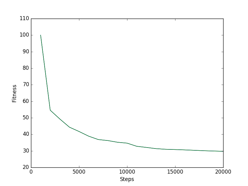
You’ll notice that the solution usually improves quickly at first, then more slowly as it converges. The shape of the curve can vary a lot based on the algorithm and parameter set. Algorithms that focus on exploitation tend to converge quickly, while those that focus on exploration tend to converge more slowly, often converging on better solutions overall. Parameter and function choices can also affect the shape of these curves. You can use these plots to answer many different questions:

1. Has the algorithm converged? If the slope is still decreasing, you probably need to relax your stop condition (i.e., run the algorithm for more steps). In my experience, this is the best way to tune your stop condition. In the example plot above, you can see that the the solution is still improving slowly, so it’s probably worth running a while longer.
2. How variable is the solution quality? That is, if you run the algorithm with the same parameter set but different random seeds, how different are the curves? Depending on your use case, consistency may be more important than finding the “best” solution.
3. How do different parameter sets (or different algorithms) compare? It’s possible to tune parameters based only on the final solution quality, but convergence curves provide additional information about how a parameterized algorithm is searching the space. Does a certain parameter combination help the algorithm explore more effectively? Does a different parameter combination help it converge quickly?
4. Is there anything wrong? If an algorithm is converging almost immediately, there’s probably something wrong with the implementation, or the mutation function you’ve chosen. Here, convergence plots can act as a simple diagnostic tool.

Conclusion

Heuristic optimization algorithms can be frustrating, especially when you’re trying to tune them. These algorithms are very flexible, which is a blessing and a curse. You can use them to solve all kinds of problems, but you pay the cost of having to tweak them quite a bit if you want something that works really well for your problem. This is the fundamental trade-off you make: few assumptions, but few guarantees. Lots of ways to customize and tune, but…. lots of ways to customize and tune.

Although it can be time-consuming, if you’re going to use an algorithm a lot, or if you really need the best solution possible, it’s worth putting some time into tuning. Fortunately, grid search, random sweeps, and convergence plots can get the job done. There are a few specific considerations to keep in mind when tuning different parameters and functions. Stay tuned (ha!) for a future post on this topic!

1 Algorithm tuning is a thing that people have studied. For very specific problems. Have they studied it for your problem? Maybe. It’s worth a look! If you can identify that your problem is fundamentally a knapsack problem, or a travelling salesman problem, or another classic well-defined problem, then a Google Scholar search can let you see what others have done, and at least get some good ideas for parameter choices and mutation functions. But even in this basic scenario, you will at least want to tune your stop conditions, since the size of your problem is likely to be different from the one studied.